This text is a compilation of selected pieces of commonly accepted mathematics and physics to be referenced in my other texts.

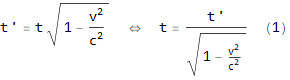
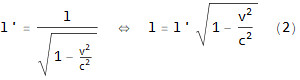
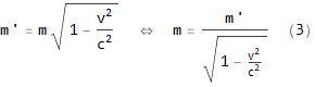
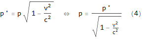
Left-side equations (1-4) are conversions for time t, distance l, moving mass m and momentum p from a stationary frame of  A-observer to a moving frame of B-observer, where corresponding quantities are time t’, distance l’, moving mass m’ and momentum p’ (which one is stationary, A or B, is a matter of taste). Right-side equations (1-4) are counter conversions from B-observer world to A-observer world. Symbol v is the velocity of the moving observer and c is the speed of light in equations.





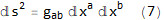
Usually it is not enough to know a simple distance l in relativistic calculations, but rather we need an exact location with coordinates x, y, z, t in space-time. Between these variables we have a differential equation 5, which defines the metric of the Lorentz-world:

Although special relativity includes formulas 3 and 4 to be used with small masses, it does not include the gravity field: special relativity assumes space to be massless. However, general relativity takes gravity into account and therefore also notices masses to exist. General relativity is defined by Einstein’s equation (equation 6):




There are several different metrics to be used with general relativity. The original metric Einstein introduced is shown on the differential equation 7:


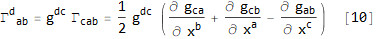
What equation 7 tells us is that all the four components of space-time, x, y, z and t, are to be treated equally manner in calculations. What is this manner is defined by the metric tensor g_ab. To find out Ricci tensor R_ab and Ricci scalar R, we must first derive from a metric tensor g_ab an expression of the Riemann curvature tensor R^d_abc (equation 8)



where notation



means Christoffel symbol (equation 10):



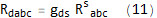
Let us write the Riemann curvature tensor as a covariant tensor R_dabc:



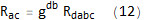
Now we get Ricci tensor R_ac



and Ricci scalar R:

German mathematician Bernhard Riemann (1826-1866 A.D.) developed a branch of mathematics called Riemann Geometry, which plants n-dimensional surfaces into the n+1 dimensional spaces called manifolds. Previously mentioned metric tensor used with the general relativity, for example, is the core of Riemann Geometry: metric tensor is the inner product defined on every point of the manifold and it changes smoothly from point to point. Metric tensor is always second rank or order i.e. it is a matrix regardless of the number of dimensions in space. One can derive the manifold curvature meter, called Riemann curvature tensor, from the second rank partial derivatives of the metric tensor. There exists numerous such tensors obeying the Gaussian curvature, but in this text collection we are only interested in those metric tensors, which form a single surface into the space and also which have constant curvature. But still there are several tensors available! For example, three dimensional space has two surface candidates fulfilling the requirements, and those are shown on figures 1 and 2:

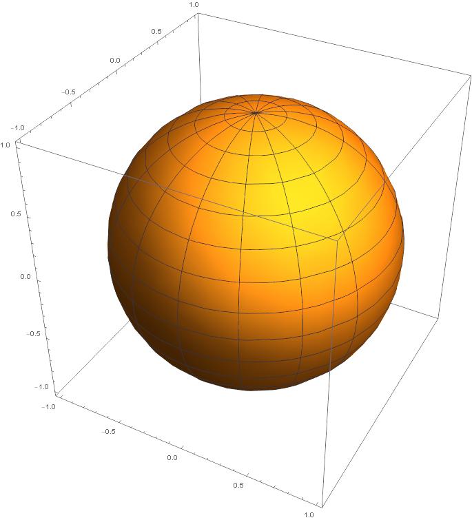
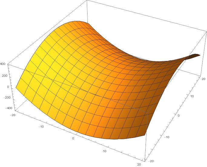
Fig. 1 The surface of the sphere is finite and unlimited.	Fig. 2. The surface of the hyperbolic paraboloid is infinite and unlimited. The surface will expand infinitely in three dimensions, but you can only see the part of the surface, which is drawn inside a box on the figure.

But because the principle of unlimited and finite requires a closed surface, only possible surface is the sphere. Therefore it is not enough for this text collection that we have a constant curvature on a single surface, but we are interested in the situation on the figure 1 only, all the way to the seventh dimension of the universe. 

Natural numbers 1, 2, 3, 4, 5, 6, ... divide into two groups: unique prime numbers and composite numbers. Prime numbers are divisible only by itself and a number 1, so prime numbers are for example 2, 3, 5, 7, 11, ... There exists infinite many prime numbers. Which ones of the natural numbers are prime and which doesn't and how primes are scattered across the composite numbers, that's the contents of analytic number theory. In practice one study prime numbers on xy-coordinate system by considering all natural numbers on x-axis while the number of found primes is the y-coordinate, as you can see here. 

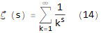
Analytic number theory is based on the Riemann Zeta-function ζ (formula 14):



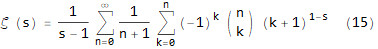
But the formula 14 is a version of Zeta-function ζ which applies only if s > 1, hence it is not suitable for analytic number theory, because all zero points lie where s < 1. We need those zero points in this text collection. Fortunately there exists another version (formula 15) of Riemann Zeta-function covering all real numbers:



The surface of absolute values drawn by function 15 includes both trivial and nontrivial zero points (as  a side note, the Riemann Hypotheses affecting on nontrivial zero points is still without a proof though Riemann himself presented it on 1859. However, that hypotheses does not have practical influence on analytic number theory). But how look like the graph in complex space drawn by function 15? Because  the function 15 is an analytic i.e. complex function, it has in fact two graphs: complex numbers are actually number of pairs and both real and imaginary parts draw their own surface to the complex space. 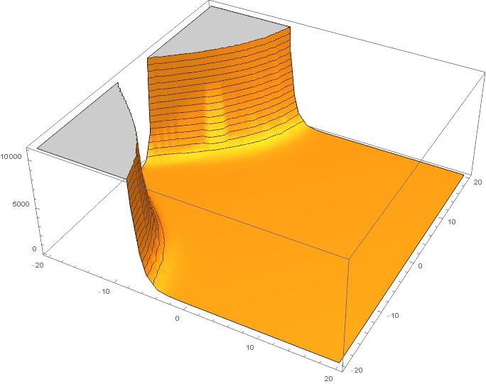If both of these surfaces penetrate the zero complex plane at a same point, then the analytic function has a zero point at that point. The surfaces drawn by function 15 are shown on figures 3, 4 and 5:

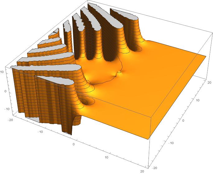
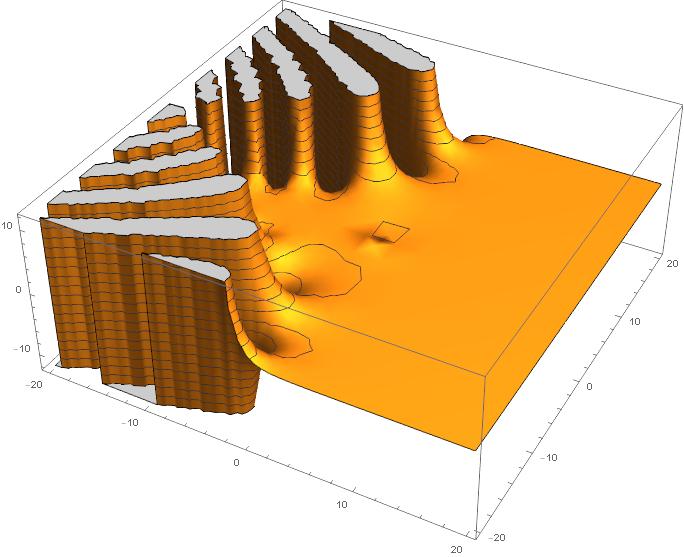
Fig. 3. The surface drawn by absolute values of Riemann Zeta-function.	Fig. 4. The surface drawn by real values of Riemann Zeta-function.	Fig. 5. The surface drawn by imaginary values of Riemann Zeta-function.